Nonadiabatic dynamics
When a molecule absorbs a photon in the UV or visible range, the energy goes to its electrons, whose configuration is changed in comparison to the ground state electronic density. The probability of absorbing a photon as a function of its wavelength - the absorption spectrum - is discussed in the page "UV excitation of molecules". Here, we will be concerned with what happens after the absorption.
The new electronic density generate right after the photon absorption does not, in general, correspond to an equilibrium state of the molecule. This means that there are forces acting on the atoms, inducing conformational changes (adiabatic process).
Dynamics simulation in the excited states is a great method for monitoring how these changes take place. You can know more about the change itself in the page "Non-adiabatic ultrafast phenomena".
There are few main challenges concerning excited state dynamics:
-
First, the potential energy of the excited state is normally much more complicated that that of the ground state. This means that we cannot use simple potential energy models as in molecular mechanics to compute the forces. Their computation should be done by solving the Schrödinger equation, which means that we have to deal with very high computational costs.
-
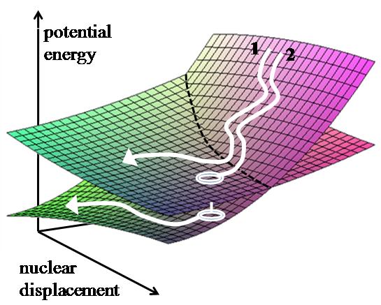
The potential energy of the electronic excited state in which the molecule is excited is often very near the potential energy of other excited states. For this reason, the molecule can jump to these other states during the relaxation (non-adiabatic process). We have also to deal with such possibility.
-
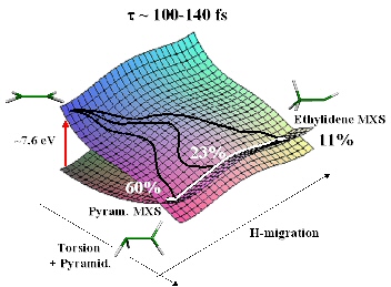
The relaxation dynamics may proceed through several different pathways. These several ways should be mapped and their relative importance evaluated.
|
|
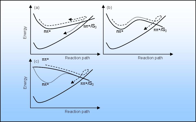
After excitation, the molecule relax in the excited state. The relaxation may occur by several different ways, as schematically illustrated for thymine [37]. |
The main method that we use in our group to investigate excited-state dynamics is the surface hopping approach, which was proposed by Tully and Preston in the early 1970's. This is a semiclassical method which allows keeping the computation costs under control. The challenges enumerated above are addressing in the following way:
-
The adiabatic processes are treated by solving the Newton's equations for the nuclei under the excited-state forces.
-
The non-adiabatic processes are treated by simultaneously computing the transition probability to other states and stochastically evaluating whether the molecule should remain in the same state or jump to another one.
-
The multiple reaction pathways are evaluated statistically by following a large number of trajectories starting with different initial conditions.
All these procedures are performed with the Newton-X program package,[23] which we have specially developed for computing surface hopping.
A bit of formalism
The basic problem in dynamics simulations of molecules is to solve the time-dependent Schrödinger equation (TDSE) for the complete molecular system,
 ,
(1)
,
(1)
where H and Y are the Hamiltonian and the wavefunction of the whole system, including nuclei and electrons.
The solution of this equation is prohibitively costly even for relatively small molecules. For this reason, we should impose a series of approximations to perform the simulations. A very common (but not unique) approach is to employ a local semiclassical approximation for the TDSE. In this approximation, the TDSE is reduced to a set of first-order differential equation for the amplitudes ck of each electronic state k:
![]() .
(2)
.
(2)
In this equation, Vk is the potential energy surface for state k, v is the nuclear velocity and Fkj is the nonadiabatic coupling vector between the states k and j, defined for each nuclei m as
![]() ,
(3)
,
(3)
where Fk is the electronic wavefunction. In equation (2), each quantity with superscript c was approximated by its value at a single nuclear configuration Rc, which is given by the Newton's equations
 .
(4)
.
(4)
In the Newton's equations, the force is given by the gradient of the electronic potential energy surfaces:
![]() .
(5)
.
(5)
The surface hopping approach
In the surface hopping approach, for a specific nuclear geometry the couplings (Eq.3) and forces (Eq.5) are computed using standard quantum chemical methods, for instance CASSCF or TDDFT. Then, Eqs. 2 and 4 are integrated numerically in one time step to obtain new amplitudes and geometries. These quantities are used to compute the hop probability from the current state l to the another state k given by:
 .
(6)
.
(6)
Based on this probability, a stochastic algorithm decides whether the molecule will remain on the same state or change to another. The procedure is repeated for a whole trajectory. Many independent trajectories are computed in order to find out what are the most important relaxation pathways.
|
|
|
|
|
Numerical nonadiabatic couplings
One of the main bottlenecks of nonadiabatic simulations is the computation of nonadiabatic couplings (Eq.3), which are not available in standard quantum chemical programs for most of quantum chemical methods. An alternative to the explicit computation of the nonadicabatic coupling vectors is to compute the time-derivative couplings, which are related to the vectors by
 .
(7)
.
(7)
The time derivative coupling can be evaluated numerically and then used in Eqs. 2 and 6. Hammes-Schiffer and Tully showed that the numerical computation of this derivative can e reduced to the computation of wavefunction overlaps along the trajectory. We have recently implemented this method to be used with MRCI, MCSCF, and TDDFT, approaches.[43,57]
Nonadiabatic dynamics with QM/MM
Nonadiabatic dynamics simulations can also profit of hybrid schemes such as QM/MM. The atoms of the entire system S to be treated by means of the hybrid method are divided into disjoint regions. For a standard QM/MM-setup with electrostatic embedding these subsets are typically an inner (I) and an outer region (O). Inner and outer region are described by quantum-mechanics and molecular mechanics, respectively. Specifically, QM electronic structure methods are used to accurately describe multiple electronic states of the compound of interest, while the MM component primarily deals with secondary environmental effects. Standard parameterized force fields are employed in the MM part incorporating bonded terms (b), van-der-Waals interactions (vdW) and electrostatic interaction (el) between partial point charges associated with each atom. The total energy of the entire system (S) is given by[54]
 (8)
(8)
Special care should be taken of the initial conditions for the dynamics. To take them from a Wigner distribution as usually done for small molecules is not practical. On the other hand, to take the initial conditions from a thermalized MM trajectory in the ground state tends to generate too cold initial ensemble for the QM region.[34,51] We have devised a way to avoid these problems by a combination of Wigner distribution for the QM part and thermal configurations for the MM part. The exact procedure is explained in Refs.[54,61].